Signal path overview

This section gives a logical overview of the signal path. The actual implementation is mathematically equivalent (when ignoring floating-point rounding errors), but it splits, combines, and reorders steps for efficiency; refer to the F-Engine Design and XB-Engine design sections for details.

Edges in diagrams are annotated to indicate the data type. The following types are used:

iN

Signed integer or fixed-point with N total bits

fN

Floating-point with N bits, following IEEE 754-2019.

cX

Complex values formed from real and imaginary components of type X e.g., cf32 is single-precision floating point complex.

Dotted boxes and arrows represent control parameters that can be adjusted at runtime.

Channelisation and delay correction

Note that the input and output bit depths (shown as i10 and ci8 on the diagram) are configurable. Between unpacking and quantisation, all calculations are performed in single precision. Since the input has a bounded range, overflow is only possible at the quantisation step (which saturates).

The figure below shows the signal path for wide-band channelisation.

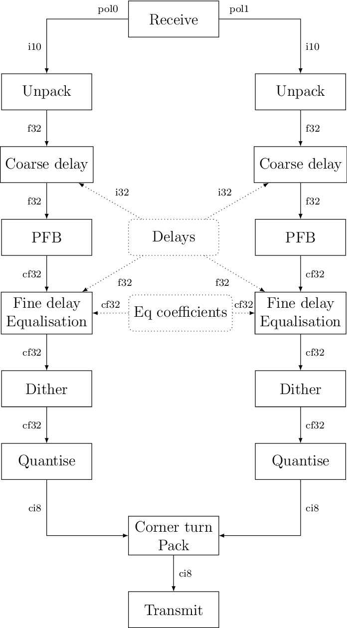
Signal path for wide-band channelisation.

Delay

Delays may be specified with sub-sample precision. To handle this, the delay is split into two components: a coarse delay (a whole number of samples) and a fine delay (between -0.5 and +0.5 samples). The coarse delay is applied as a shift in time, while the fine delay is applied as a phase slope in the frequency domain. As noted in Delay and phase compensation, the user provides the overall phase adjustment for the centre frequency, and the constant term of the phase slope is computed from that (taking into account the effect of the coarse delay on phase).

The fine delay and the fixed phase offset for each spectrum are computed in double precision then reduced to single precision for application. Conversion of the delay to a per-channel phase correction, and of phases to complex phasors are done in single precision.

Polyphase filter bank (PFB)

A finite impulse response (FIR) filter is applied to the signal to condition the frequency-domain response. The filter is the product of a window function (to reduce spectral leakage) and a sinc (to broaden the peak to cover the frequency bin). Specifically, if there are \(n\) output channels and \(t\) taps in the polyphase filter bank, then the filter has length \(w = 2nt\), with coefficients

\[x_i = AW_i\operatorname{sinc}\left(w_c\cdot \frac{i + \tfrac 12 - nt}{2n}\right),\]

where \(i\) runs from 0 to \(w - 1\), and \(W\) is the window function, for which there are two choices:

• Hann: \(W_i = \sin^2\left(\frac{\pi i}{w - 1}\right)\)

• Rect: \(W_i = 1\).

\(A\) is a normalisation factor which is chosen such that \(\sum_i x_i^2 = 1\). This ensures that given white Gaussian noise as input, the expected output power in a channel is the same as the expected input power in a digitised sample. Note that the input and output are treated as integers rather than as fixed-point values.

The tuning parameter \(w_c\) (specified by the --w-cutoff command-line option) scales the width of the response in the frequency domain. The default value is 1, which makes the width of the response (at -6dB) approximately equal the channel spacing.

In some cases spectral leakage is less important than the ability to reconstruct the original signal. Setting \(t = 1\), \(w_c = 0\) and using the rectangular window function gives a degenerate PFB in which each block of \(2n\) samples is Fourier transformed.

Dithering

To improve linearity, a random value selected uniformly from the interval (-0.5, 0.5) is added to each component (real and imaginary) before quantisation. The random seeds are carefully chosen to ensure that random sequences are not shared across antennas.

Narrowband

Narrowband outputs are those in which only a portion of the digitised bandwidth is channelised and output. Typically they have narrower channel widths. The overall approach is as follows:

1. The signal is multiplied (mixed) by a complex tone of the form \(e^{2\pi jft}\), to effect a shift in the frequency of the signal. The centre of the desired band is placed at the DC frequency.

2. The signal is convolved with a low-pass filter. This suppresses most of the unwanted parts of the band, to the extent possible with a FIR filter.

3. The signal is subsampled (every Nth sample is retained), reducing the data rate. The low-pass filter above limits aliasing. At this stage, twice as much bandwidth as desired is retained. The steps up to this one are referred to as digital down-conversion (DDC).

4. The coarse delay and PFB proceed largely as before, but using double the final channel count (since the bandwidth is also doubled, the channel width is as desired). The input is now complex rather than real (due to the mixing), so the PFB is complex-to-complex rather than real-to-complex.

5. Half the channels (the outer half) are discarded.

Note

To avoid confusion, the “subsampling factor” is the ratio of original to retained samples in the subsampling step, while the “decimation factor” is the factor by which the bandwidth is reduced. Because the mixing turns a real signal into a complex signal, the subsampling factor is twice the decimation factor in step 3 (but equal to the overall decimation factor).

The decimation is thus achieved by a combination of time-domain (steps 2 and 3) and frequency domain (step 5) techniques. This has better computational efficiency than a purely frequency-domain approach (which would require the PFB to be run on the full bandwidth), while mitigating many of the filter design problems inherent in a purely time-domain approach (the roll-off of the FIR filter can be hidden in the discarded outer channels).

The figure below shows the modified signal path.

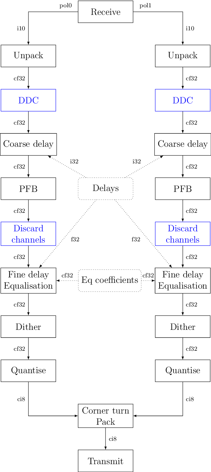
Signal path for narrow-band channelisation (with new stages in blue).

Discarding half the channels after channelisation allows for a lot of freedom in the design of the DDC FIR filter: the discarded channels can have an arbitrary response. This allows for a gradual transition from passband to stopband. We use scipy.signal.remez() to produce a filter that is as close as possible to 1 in the passband and 0 in the stopband. A weighting factor (which the user can override) balances the priority of the passband (ripple) and stopband (alias suppression).

The filter performance is slightly improved by noting that the discarded channels have multiple aliases, and the filter response in those aliases is also irrelevant. We thus use scipy.signal.remez() to only optimise the response to those channels that alias into the output.

Narrowband without discard

The above combined time-frequency approach to narrowband can be disabled, giving a purely time-domain FIR filter. In this case, step 5 is skipped. The primary use case is for reconstructing a time-domain signal from the channelised output, where completely discarding channels appears to lose necessary information.

The filter design in this case is more critical, and needs to trade off factors such as passband ripple, roll-off, and alias rejection. The user provides the desired pass bandwidth. We then use scipy.signal.remez() with the stop bandwidth calculated such that the roll-off is symmetrically located around the Nyquist frequency. This means that after subsampling, half of the roll-off region will alias, but it will not alias with the passband. As before, users can override a weighting factor that balances the priority of the passband and stopband.

It may be possible to improve this further by leaving other aliases of the roll-off region unconstrained, as was done above, but this has not currently been investigated.

Correlation

Given a baseline (p, q) and time-varying channelised voltages \(e_p\) and \(e_q\), the correlation product is the sum of \(e_p \overline{e_q}\) over the accumulation period. This is computed in integer arithmetic and so is lossless except when saturation occurs.

The figure below shows the signal path.

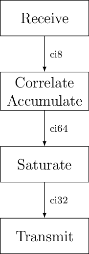
Signal path for correlation

Beamforming

The signal path below is repeated for each single-polarisation beam. Delays are computed purely with a phase slope in the frequency domain, similarly to the fine delays in the channeliser. Dithering is done the same way as for channelisation. Since all calculations are performed in single precision floating point and the input has a limited range, overflow can only occur during quantisation (which saturates).

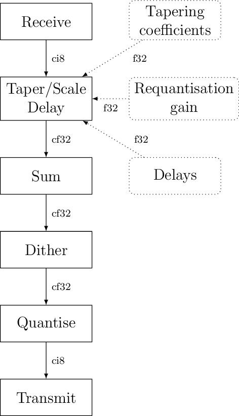
Signal path for beamforming